Advanced Clustering and Prediction techniques

Machine Learning

Employing sophisticated clustering techniques with retail customer data and comparing further with prediction models

Author

Affiliation

Published

November 24, 2023

Advanced Clustering and Prediction techniques Using Retail Customer Data

Employing sophisticated clustering techniques with retail customer data and comparing further with prediction models

Clustering is a fundamental technique in machine learning that involves grouping data points so that the objects in the same group (or cluster) are more similar to each other than to those in other groups. It’s a form of unsupervised learning, as the groups are not predefined but rather determined by the algorithm itself. This approach is particularly useful in understanding the structure within data, identifying patterns, and making strategic decisions.

In this blog, we will explore how to apply clustering techniques to a customer dataset. Our dataset contains customer information with attributes like Customer ID, Age, Annual Income, and Spending Score. The goal is to segment customers into distinct groups based on these features, which can help in tailoring marketing strategies, understanding customer behavior, and improving customer service.

Introduction

Data Loading and Basic Visualization

# Importing libraries
import pandas as pd
import matplotlib.pyplot as plt
import seaborn as sns
from sklearn.cluster import KMeans
from sklearn.preprocessing import StandardScaler

# Load the dataset
customer_df = pd.read_csv('clusteringCustomerData.csv')
print(customer_df.head())

   CustomerID  Age  Annual_Income  Spending_Score
0           1   62             75              81
1           2   65             76              23
2           3   18             98              80
3           4   21             48              90
4           5   21             47               9

Exploring Data Analysis

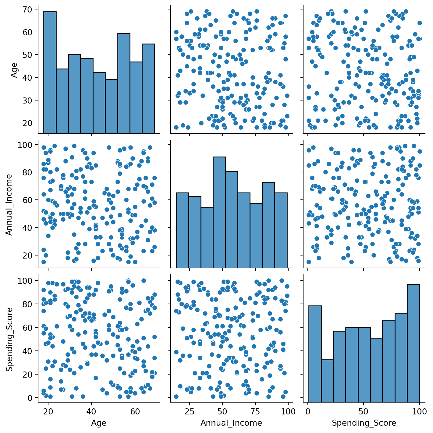
#Visualize the distributions and relationships between features.
sns.pairplot(customer_df.drop('CustomerID', axis=1))
plt.show()

Data Preprocessing

#Encoding categorical data and scaling features.
#Standardize the data.
# Selecting features to be scaled
features = customer_df[['Age', 'Annual_Income', 'Spending_Score']]

# Standardizing the features
scaler = StandardScaler()
scaled_features = scaler.fit_transform(features)

# Converting scaled features back to a DataFrame
scaled_features_df = pd.DataFrame(scaled_features, columns=features.columns)

# Displaying the first few rows of the scaled data
print(scaled_features_df.head())

        Age  Annual_Income  Spending_Score
0  1.237684       0.746278        0.901945
1  1.428146       0.788416       -1.020966
2 -1.555756       1.715469        0.868791
3 -1.365294      -0.391469        1.200327
4 -1.365294      -0.433608       -1.485117

Exploratory Data Analysis (EDA)

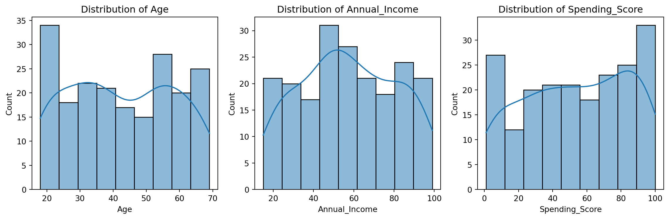
Beyond basic visualizations, we’ll use EDA to understand the data distributions and potential relationships.

# Visualizing the distribution of features
plt.figure(figsize=(12, 4))
for i, col in enumerate(['Age', 'Annual_Income', 'Spending_Score']):
    plt.subplot(1, 3, i+1)
    sns.histplot(customer_df[col], kde=True)
    plt.title(f'Distribution of {col}')
plt.tight_layout()
plt.show()

Advanced Clustering with Multiple Techniques

We’ll explore different clustering algorithms beyond K-Means, such as Hierarchical Clustering and DBSCAN, to understand how they segment the data differently.

1. K-Means Clustering

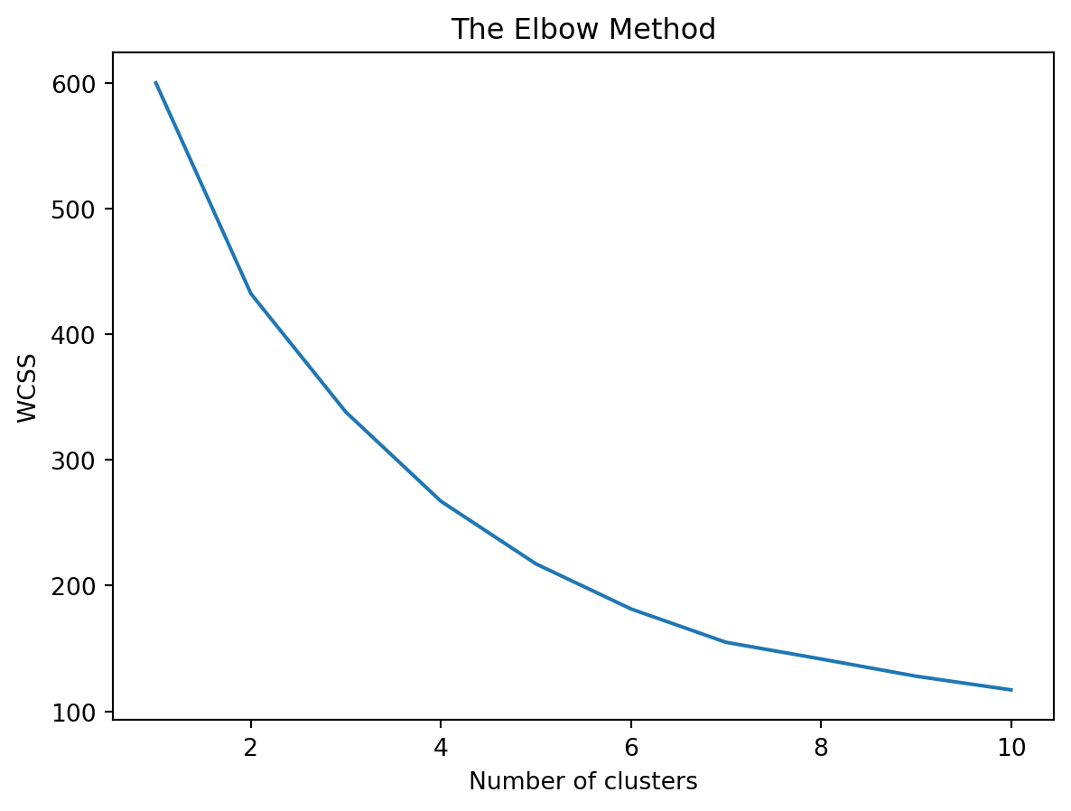
#Using the Elbow Method to determine the optimal number of clusters.
wcss = []
for i in range(1, 11):
    kmeans = KMeans(n_clusters=i, n_init=10, random_state=42)
    kmeans.fit(scaled_features)
    wcss.append(kmeans.inertia_)
    customer_df['KMeans_Cluster'] = kmeans.labels_
plt.plot(range(1, 11), wcss)
plt.title('The Elbow Method')
plt.xlabel('Number of clusters')
plt.ylabel('WCSS')
plt.show()

Application of K-Means

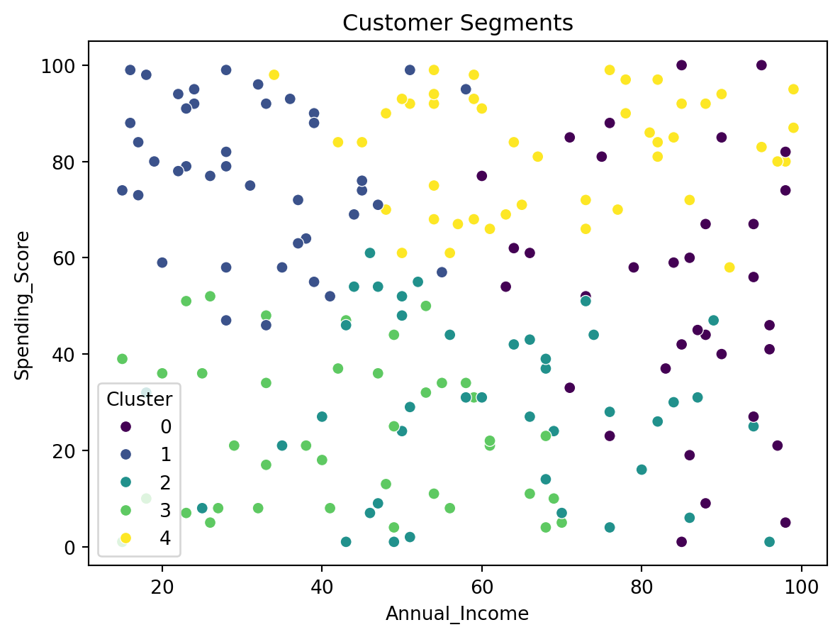
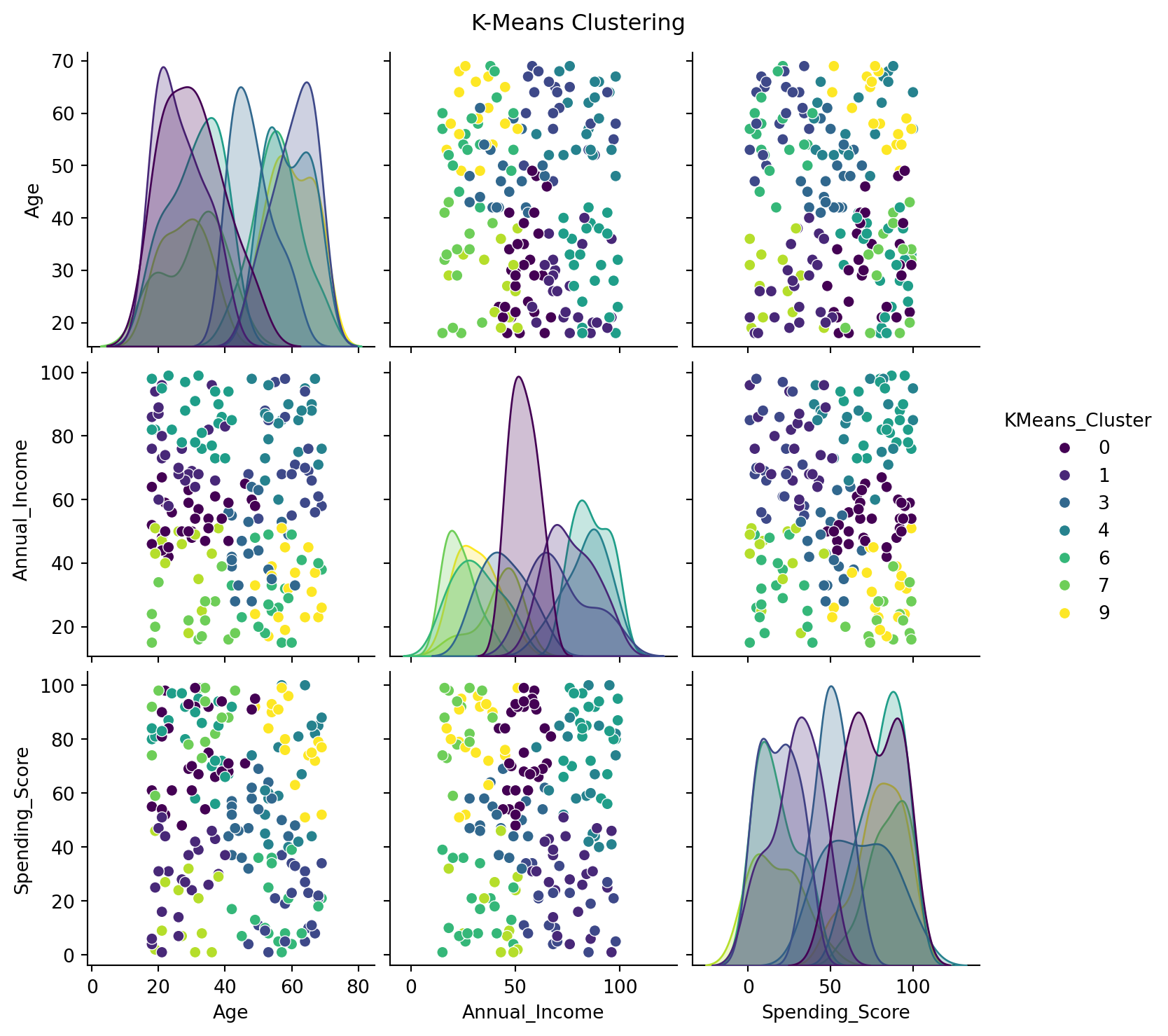
#Applying K-Means and visualizing the clusters.
kmeans = KMeans(n_clusters=5, n_init=10, random_state=42)
customer_df['Cluster'] = kmeans.fit_predict(scaled_features)
sns.scatterplot(x='Annual_Income', y='Spending_Score', hue='Cluster', data=customer_df, palette='viridis')
plt.title('Customer Segments')
plt.show()

K-Means Visualization

sns.pairplot(customer_df, vars=['Age', 'Annual_Income', 'Spending_Score'], hue='KMeans_Cluster', palette='viridis')
plt.suptitle('K-Means Clustering', y=1.02)
plt.show()

2. DBSCAN clustering

from sklearn.cluster import DBSCAN

# DBSCAN clustering
dbscan = DBSCAN(eps=0.5, min_samples=5).fit(scaled_features_df)
customer_df['DBSCAN_Cluster'] = dbscan.labels_

Density-Based Spatial Clustering of Applications with Noise (DBSCAN) Visualization

# Visualizing DBSCAN Clusters
sns.scatterplot(x='Annual_Income', y='Spending_Score', hue='DBSCAN_Cluster', data=customer_df, palette='viridis')
plt.title('DBSCAN Clustering')
plt.show()

3. Hierarchical Cluster Visualization

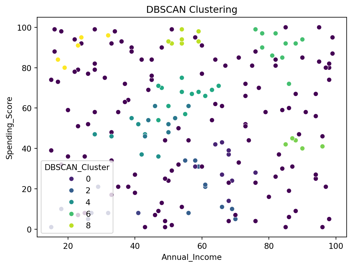
Visualize the clusters formed by each algorithm in multiple dimensions to gain deeper insights.

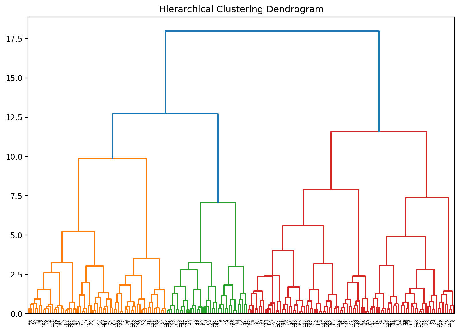
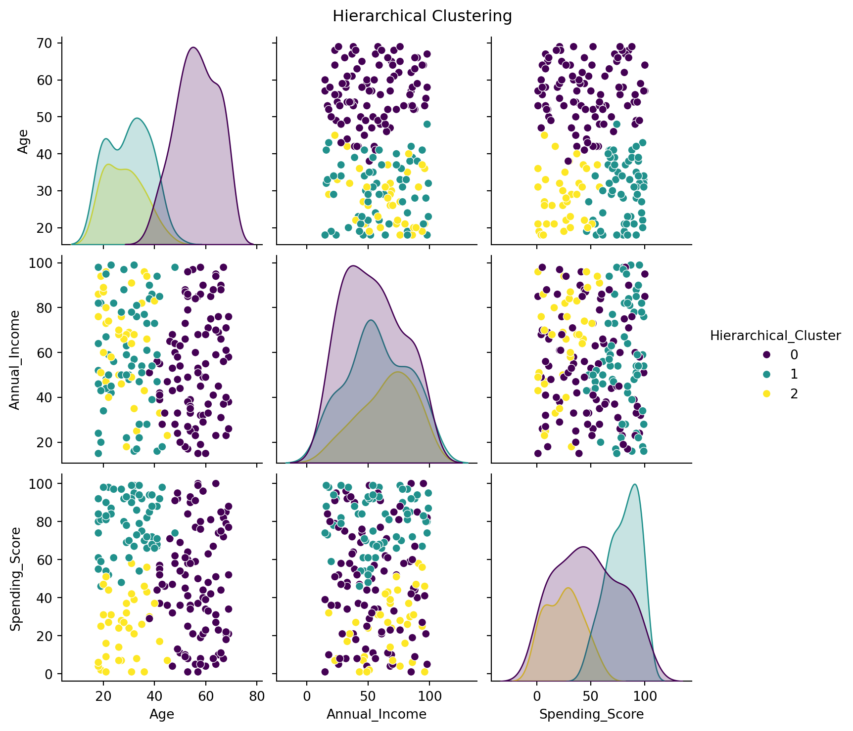
from scipy.cluster.hierarchy import dendrogram, linkage
from sklearn.cluster import AgglomerativeClustering  # Import AgglomerativeClustering

# Performing Hierarchical Clustering
linked = linkage(scaled_features_df, method='ward')

# Plotting the Dendrogram
plt.figure(figsize=(10, 7))
dendrogram(linked, orientation='top', distance_sort='descending', show_leaf_counts=True)
plt.title('Hierarchical Clustering Dendrogram')
plt.show()

# Perform hierarchical clustering and add the cluster labels to customer_df
clustering = AgglomerativeClustering(n_clusters=3)  # Specify the number of clusters
customer_df['Hierarchical_Cluster'] = clustering.fit_predict(scaled_features_df)

# Hierarchical Clustering Visualization
sns.pairplot(customer_df, vars=['Age', 'Annual_Income', 'Spending_Score'], hue='Hierarchical_Cluster', palette='viridis')
plt.suptitle('Hierarchical Clustering', y=1.02)
plt.show()

Hierarchical Clustering Cut

from scipy.cluster.hierarchy import fcluster

# Cutting the Dendrogram to form clusters
customer_df['Hierarchical_Cluster'] = fcluster(linked, t=3, criterion='maxclust')

sns.scatterplot(data=customer_df, x='Annual_Income', y='Spending_Score', hue='Hierarchical_Cluster', palette='viridis')
plt.title('Hierarchical Clustering')
plt.show()

Silhouette Analysis for K-means and Hierarchical Clustering

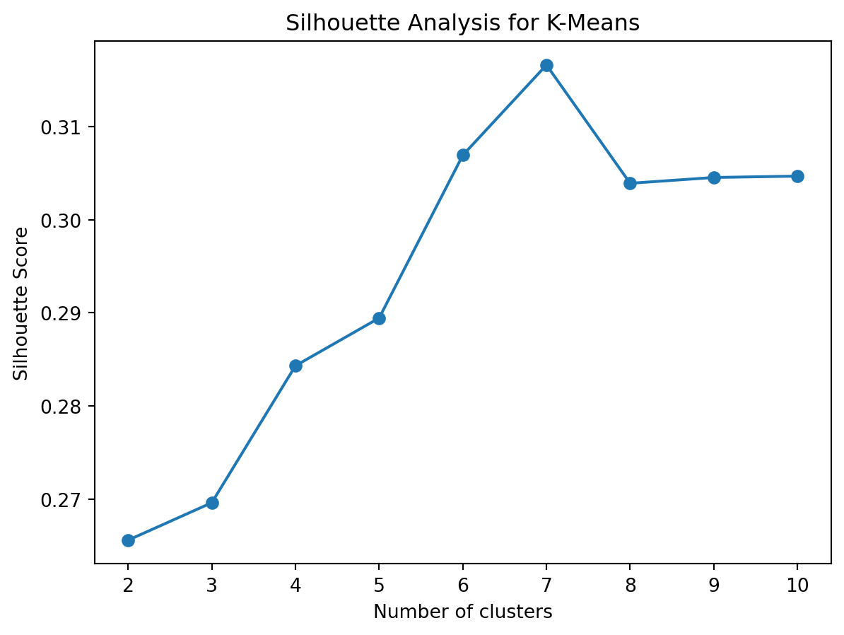
1. K-Means Clustering

from sklearn.metrics import silhouette_samples, silhouette_score
import numpy as np

# Calculate silhouette scores for different cluster numbers
silhouette_scores = []
for n_clusters in range(2, 11):
    kmeans = KMeans(n_clusters=n_clusters, n_init=10, random_state=42)
    cluster_labels = kmeans.fit_predict(scaled_features)
    silhouette_avg = silhouette_score(scaled_features, cluster_labels)
    silhouette_scores.append(silhouette_avg)

# Plot silhouette scores
plt.plot(range(2, 11), silhouette_scores, marker='o')
plt.title('Silhouette Analysis for K-Means')
plt.xlabel('Number of clusters')
plt.ylabel('Silhouette Score')
plt.show()

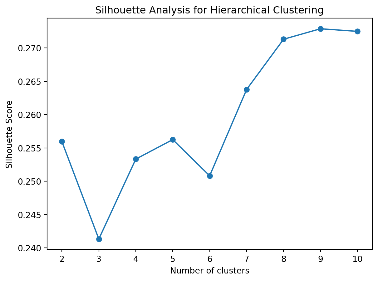
2. Hierarchical Clustering

from sklearn.cluster import AgglomerativeClustering

# Calculate silhouette scores for different cluster numbers in hierarchical clustering
silhouette_scores_hierarchical = []
for n_clusters in range(2, 11):
    hierarchical = AgglomerativeClustering(n_clusters=n_clusters)
    cluster_labels = hierarchical.fit_predict(scaled_features)
    silhouette_avg = silhouette_score(scaled_features, cluster_labels)
    silhouette_scores_hierarchical.append(silhouette_avg)

# Plot silhouette scores for hierarchical clustering
plt.plot(range(2, 11), silhouette_scores_hierarchical, marker='o')
plt.title('Silhouette Analysis for Hierarchical Clustering')
plt.xlabel('Number of clusters')
plt.ylabel('Silhouette Score')
plt.show()

Conclusion

#In this in-depth analysis, we have explored different clustering techniques and visualized their results to segment customers in a comprehensive manner. Each method offers unique insights: K-Means provides clear segmentations, Hierarchical Clustering helps us understand the data structure, and DBSCAN identifies core and outlier points effectively.

By comparing these methods, we can choose the one that best suits our specific needs for customer segmentation. This advanced clustering analysis can guide strategic decisions, improve customer engagement, and enhance targeting in marketing campaigns.

Reuse

https://creativecommons.org/licenses/by/4.0/