Robot Control
Compliant Joints
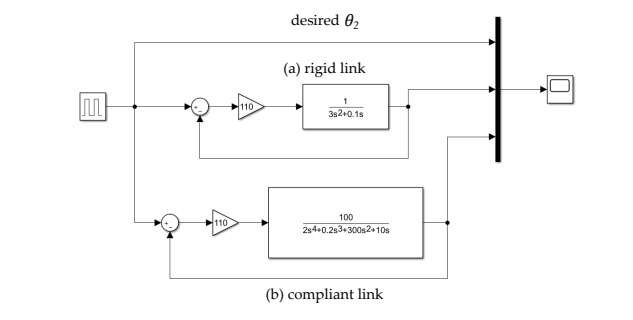
Now we are simulating the rigid system and compliant system in Simulink (Matlab). For both systems set \(\normalsize \theta_𝑑\) as a Pulse Generator with amplitude 1 m, period 5 s, and pulse width 50%. The model stop time should be 50 s. Here we are simulating two separate plots.
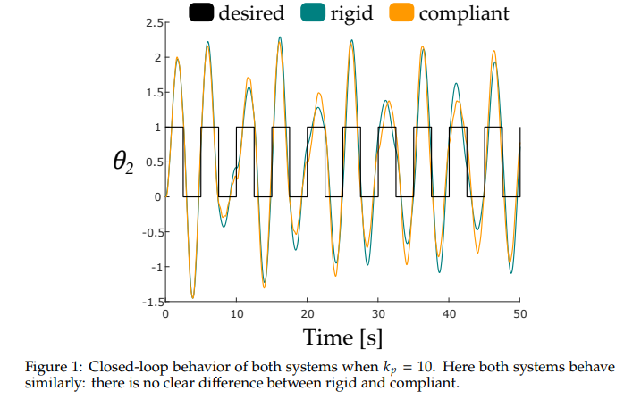
One plot should show \(\normalsize \theta_𝑑, \, \theta_2\) (for the rigid system) and 𝜃2 (for the compliant system) when \(\normalsize 𝑘_𝑝 = 10\). The other plot should show \(\normalsize \theta_𝑑, \, \theta_2\) (for the rigid system) and 𝜃2 (for the compliant system) when \(\normalsize 𝑘_𝑝 = 110\), including labels and captions.
Simulink model:
Result:
- Closed-loop behavior of both systems when \(\normalsize 𝑘_𝑝 = 10\).
- Closed-loop behavior of both systems when \(\normalsize 𝑘_𝑝 = 110\).
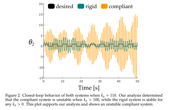
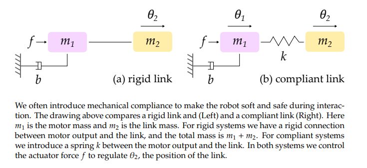
Does introducing compliance (e.g., the spring between the motor and link) make it easier or harder to control the robot?
Compliance makes it harder to control the system. Our analysis shows that the added compliance restricts the range of 𝑘𝑝 for which the system is stable. Physically, the added spring causes the second mass to oscillate, and the controllers we design must work to mitigate these oscillations.
Multivariable Control
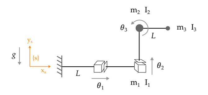
In this problem, we will simulate control the robot shown above. We have already obtained the dynamics of this robot (which are the mass, coriolis matrices and the gravity vector) which is mentioned in the code below. The robot starts at joint position \(\normalsize \theta = 0\).
Here \(\normalsize 𝐿 = 1, 𝑚_1 = 𝑚_2 = 𝑚_3 = 1, and \, 𝐼_3 = 0.1.\)
Using the given simulation parameters and frame rates as required, we are modifing the code as needed so that the robot reaches for \(\normalsize \theta_d\) using multivariable PD control with gravity compensation:
\(\normalsize \tau = 𝐾_𝑃(\theta_𝑑 − \theta) − 𝐾_𝐷 \dot\theta + 𝑔(\theta)\)
- CASE 1: A simulation where \(\normalsize 𝐾_P = 𝐼\) and \(\normalsize 𝐾_𝐷 = 𝐼\). Let the desired position be:
\[\normalsize \theta_d = \left(\begin{array}{cc} -2\\ 2\\ \pi/4 \end{array}\right) \]
Implementation
MATLAB Code
close all
clear
clc

% create figure
figure
axis([-4, 4, -4, 4])
grid on
hold on

% save as a video file
v = VideoWriter('Multivariable_1.mp4', 'MPEG-4');
v.FrameRate = 100;
open(v);

% pick your system parameters
m1 = 1;
m2 = 1;
m3 = 1;
I3 = 0.1;
L = 1;
g = 9.81;
deltaT = 0.01;

% initial conditions
theta = [0; 0; 0];
thetadot = [0; 0; 0];
thetadotdot = [0; 0; 0];
time = 0;

% forward kinematics to end-effector
S1 = [0;0;0;1;0;0];
S2 = [0;0;0;0;1;0];
S3 = [0;0;1;0;-L;0];
S = [S1, S2, S3];
M3 = [eye(3), [2*L;0;0]; 0 0 0 1];

% For CASE 1
Kp = eye(3);
Kd = eye(3);

M0 = [eye(3), [L;0;0]; 0 0 0 1];
M1 = [eye(3), [L;0;0]; 0 0 0 1];
M2 = [eye(3), [L;0;0]; 0 0 0 1];

for idx = 1:1000

    % get desired position
    theta_d = [-2; 2; pi/4];
    thetadot_d = [0; 0; 0];
    T_d = fk(M3, [S1 S2 S3], theta_d);

    % plot the robot
    p0 = [0; 0];
    T1 = fk(M1, S1,theta(1:1,:));
    p1 = T1(1:2,4);                         % position of end of link 1
    T2 = fk(M2,[S1 S2],theta(1:2,:));
    p2 = T2(1:2,4);                         % position of end of link 2
    T3 = fk(M3,[S1 S2 S3],theta(1:3,:));
    p3 = T3(1:2,4);                         % position of end of link 3
    P = [p0, p1, p2, p3];
    cla;
    plot(P(1,:), P(2,:), 'o-', 'color',[1, 0.5, 0],'linewidth',4)

    % plot the desired position
    plot(T_d(1,4), T_d(2,4), 'ok', 'MarkerFaceColor','k')
    drawnow
    frame = getframe(gcf);
    writeVideo(v,frame);

    % Mass matrix
    M = [m1 + m2 + m3, 0, -L*m3*sin(theta(3));
            0, m2 + m3, L*m3*cos(theta(3));
            -L*m3*sin(theta(3)), L*m3*cos(theta(3)), m3*L^2 + I3];

    % Coriolis matrix
    C = [0, 0, -L*thetadot(3)*m3*cos(theta(3));
        0, 0, -L*thetadot(3)*m3*sin(theta(3));
        0, 0,                 0];

    % Gravity vector
    G = [0; g*m2 + g*m3; L*g*m3*cos(theta(3))];

    % Choose your controller tau (Just for reference and knowledge)
    e1 =    theta_d - theta;
    e1dot = thetadot_d - thetadot;

    % Reference from a journal and a book (Modern Robotics)
    tau = Kp*(theta_d-theta) + Kd*(thetadot_d - thetadot) + G;

    % integrate to update velocity and position
    thetadotdot = M \ (tau - C*thetadot - G);
    thetadot = thetadot + deltaT * thetadotdot;
    theta = theta + deltaT * thetadot;
    time = time + deltaT;

end

close(v);
close all
Result:

- CASE 2: Reaching for the same \(\normalsize \theta_d\) as in the previous part, but now we are tuning \(\normalsize 𝐾_𝑃\) and \(\normalsize 𝐾_𝐷\) to improve the robot’s performance, thus making a simulation with our best performing gains.
\[\normalsize \theta_d = \left(\begin{array}{cc} -2\\ 2\\ \pi/4 \end{array}\right) \]
And here we choose our gains to be:
\(\normalsize K_p = eye(3)*25\)
\(\normalsize K_d = eye(3)*25\)
Implementation
MATLAB Code
close all
clear
clc

% create figure
figure
axis([-4, 4, -4, 4])
grid on
hold on

% save as a video file
v = VideoWriter('Multivariable_2.mp4', 'MPEG-4');
v.FrameRate = 100;
open(v);

% pick your system parameters
m1 = 1;
m2 = 1;
m3 = 1;
I3 = 0.1;
L = 1;
g = 9.81;
deltaT = 0.01;

% initial conditions
theta = [0; 0; 0];
thetadot = [0; 0; 0];
thetadotdot = [0; 0; 0];
time = 0;

% forward kinematics to end-effector
S1 = [0;0;0;1;0;0];
S2 = [0;0;0;0;1;0];
S3 = [0;0;1;0;-L;0];
S = [S1, S2, S3];
M3 = [eye(3), [2*L;0;0]; 0 0 0 1];

% For CASE 2 (Our best gains that yields the best and the most stable result)
Kp = eye(3)*25;
Kd = eye(3)*25;

M0 = [eye(3), [L;0;0]; 0 0 0 1];
M1 = [eye(3), [L;0;0]; 0 0 0 1];
M2 = [eye(3), [L;0;0]; 0 0 0 1];

for idx = 1:1000

    % get desired position
    theta_d = [-2; 2; pi/4];
    thetadot_d = [0; 0; 0];
    T_d = fk(M3, [S1 S2 S3], theta_d);

    % plot the robot
    p0 = [0; 0];
    T1 = fk(M1, S1,theta(1:1,:));
    p1 = T1(1:2,4);                         % position of end of link 1
    T2 = fk(M2,[S1 S2],theta(1:2,:));
    p2 = T2(1:2,4);                         % position of end of link 2
    T3 = fk(M3,[S1 S2 S3],theta(1:3,:));
    p3 = T3(1:2,4);                         % position of end of link 3
    P = [p0, p1, p2, p3];
    cla;
    plot(P(1,:), P(2,:), 'o-', 'color',[1, 0.5, 0],'linewidth',4)
    % plot the desired position
    plot(T_d(1,4), T_d(2,4), 'ok', 'MarkerFaceColor','k')
    drawnow
    frame = getframe(gcf);
    writeVideo(v,frame);

    % mass matrix
    M = [m1 + m2 + m3, 0, -L*m3*sin(theta(3));
            0, m2 + m3, L*m3*cos(theta(3));
            -L*m3*sin(theta(3)), L*m3*cos(theta(3)), m3*L^2 + I3];

    % Coriolis matrix
    C = [0, 0, -L*thetadot(3)*m3*cos(theta(3));
        0, 0, -L*thetadot(3)*m3*sin(theta(3));
        0, 0,                 0];

    % Gravity vector
    G = [0; g*m2 + g*m3; L*g*m3*cos(theta(3))];

    % Choose your controller tau (Just for reference and knowledge)
    e1 =    theta_d - theta;
    e1dot = thetadot_d - thetadot;

    % Reference from a journal and a book (Modern Robotics)
    tau = Kp*(theta_d-theta) + Kd*(thetadot_d - thetadot) + G;

    % integrate to update velocity and position
    thetadotdot = M \ (tau - C*thetadot - G);
    thetadot = thetadot + deltaT * thetadotdot;
    theta = theta + deltaT * thetadot;
    time = time + deltaT;

end

close(v);
close all
Result:
- CASE 3: Controlling the robot to move in a circle. Let 𝑡 be the simulation time (variable time in the code), and define the desired trajectory as:
\[\normalsize \theta_d = \left(\begin{array}{cc} 2\cos(0.5\pi t)\\ 2\sin(0.5\pi t)\\ \pi/2 \end{array}\right) \]
\[\normalsize \dot\theta_d = \left(\begin{array}{cc} -\pi\sin(0.5\pi t)\\ \pi\cos(0.5\pi t)\\ 0 \end{array}\right) \]
And here we still keep our best gains:
\(\normalsize K_p = eye(3)*25\)
\(\normalsize K_d = eye(3)*25\)
Implementation
MATLAB Code
close all
clear
clc

% create figure
figure
axis([-4, 4, -4, 4])
grid on
hold on

% save as a video file
v = VideoWriter('Multivariable_3.mp4', 'MPEG-4');
v.FrameRate = 100;
open(v);

% pick your system parameters
m1 = 1;
m2 = 1;
m3 = 1;
I3 = 0.1;
L = 1;
g = 9.81;
deltaT = 0.01;

% initial conditions
theta = [0; 0; 0];
thetadot = [0; 0; 0];
thetadotdot = [0; 0; 0];
time = 0;

% forward kinematics to end-effector
S1 = [0;0;0;1;0;0];
S2 = [0;0;0;0;1;0];
S3 = [0;0;1;0;-L;0];
S = [S1, S2, S3];
M3 = [eye(3), [2*L;0;0]; 0 0 0 1];

% For CASE 3
Kp = eye(3)*25;
Kd = eye(3)*25;

M0 = [eye(3), [L;0;0]; 0 0 0 1];
M1 = [eye(3), [L;0;0]; 0 0 0 1];
M2 = [eye(3), [L;0;0]; 0 0 0 1];

for idx = 1:1000

    % get desired position
    theta_d = [2*cos(pi*time/2); 2*sin(pi*time/2); pi/2];
    thetadot_d = [-pi*sin(pi*time/2); pi*cos(pi*time/2); 0];
    T_d = fk(M3, [S1 S2 S3], theta_d);

    % plot the robot
    p0 = [0; 0];
    T1 = fk(M1, S1,theta(1:1,:));
    p1 = T1(1:2,4);                         % position of end of link 1
    T2 = fk(M2,[S1 S2],theta(1:2,:));
    p2 = T2(1:2,4);                         % position of end of link 2
    T3 = fk(M3,[S1 S2 S3],theta(1:3,:));
    p3 = T3(1:2,4);                         % position of end of link 3
    P = [p0, p1, p2, p3];
    cla;
    plot(P(1,:), P(2,:), 'o-', 'color',[1, 0.5, 0],'linewidth',4)
    % plot the desired position
    plot(T_d(1,4), T_d(2,4), 'ok', 'MarkerFaceColor','k')
    drawnow
    frame = getframe(gcf);
    writeVideo(v,frame);

    % mass matrix
    M = [m1 + m2 + m3, 0, -L*m3*sin(theta(3));
            0, m2 + m3, L*m3*cos(theta(3));
            -L*m3*sin(theta(3)), L*m3*cos(theta(3)), m3*L^2 + I3];

    % Coriolis matrix
    C = [0, 0, -L*thetadot(3)*m3*cos(theta(3));
        0, 0, -L*thetadot(3)*m3*sin(theta(3));
        0, 0,                 0];

    % Gravity vector
    G = [0; g*m2 + g*m3; L*g*m3*cos(theta(3))];

    % Choose your controller tau (Just for reference and knowledge)
    e1 =    theta_d - theta;
    e1dot = thetadot_d - thetadot;

    % Reference from a journal and a book (Modern Robotics)
    tau = Kp*(theta_d-theta) + Kd*(thetadot_d - thetadot) + G;

    % integrate to update velocity and position
    thetadotdot = M \ (tau - C*thetadot - G);
    thetadot = thetadot + deltaT * thetadotdot;
    theta = theta + deltaT * thetadot;
    time = time + deltaT;

end

close(v);
close all
Result: